Lesson 3: How we describe data

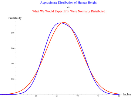
Large piles of data can be summarized and described many ways. This lesson will cover a few important ones: distribution, average, and standard deviation.

The data distribution is a description of how the data is spread out through parameter space. It tells us the probability of finding a data point with a specific value. The best known distribution is the normal or Gaussian distribution, which is often described as a "bell curve". Some pictures will make this clearer.

Here is some made up data from a study where the number of cats in each home was determined for 1000 homes. Because cats per house is a discrete variable we use a bar graph. You can see a curved distribution (imagine a line connecting the tops of the bars; it's like a hill), and can see that about 250/1000 homes, or 25% had 1 cat. From this we can say that if we picked a house from the study at random and visited it, there is a 25% chance we'd find 1 cat living there. This distribution is skewed left from normal (since no one has fewer than zero cats). Skew describes the level of asymmetry of a distribution: how much longer or fatter one "tail" is than the other.

Image from askamathematician.com

Here is some less made up data regarding the height of college students (male and female). This distribution is almost normal (a true normal distribution is in red). This distribution uses a line because height is a continuous variable. We can see that the probability of being 60" (5'0") is about 2.2%. How normally the data is distributed can have important impacts on how valid different statistical tests of a sample are. You'll start to see this when I talk about different types of averages.

In lay terms we all know what an average is; the formal definition is that an average is a measure of central tendency and can be described by the mean, median, or mode of a data set (sample or population). However, in most cases average refers to the arithmetic mean of a data set (population or sample). The arithmetic mean is the sum of all the values in the set divided by the number of values in the set. On a data distribution plot the mean is at the "hill top" only when the data is normally distributed (no skew); in a skewed distribution the mean will favor the "fat tailed" end of the distribution. There are other types of means (Pythagorean, geometric, and harmonic), but those aren't important to us now.

The next way to describe the average of a data set is with the median. Median is the middle value. By definition 50% of the values will be above the median and 50% below (unless a large number of values are equal to the median). On a data distribution plot the median is at the "hill top" only when the data is normally distributed (no skew); in a skewed distribution the median will favor the "fat tailed" end of the distribution, but far less dramatically than the mean. This gives median a special advantage for researchers, as the median value of a data set is less susceptible to influence from a single extreme, outlier value.

The final type of average is the mode. Mode is the most common value in a data set. On a data distribution plot the mode will always be at the "hill top" regardless of skew. This gives me an excuse to introduce the term bimodal. A bimodal distribution, as the name suggests, is a distribution with two modes or two hill tops (for a data set to really have two modes the two peaks must be equal, otherwise the bimodal distribution will have two peaks but mathematically the mode will be the top of the higher hill).

Let's go back to our cat study and see how these values compare. This time I didn't lump all families with 5 or more cats together.

Mean - 2.01 cats

Median - 2 cats

Mode - 1 cat




If we imagine that one family had 1000 cats, then only the mean changes. The mean becomes 3. In this case, because the data set is large the mean is fairly robust to one extreme value, but the median and mode are more so. (If we only sampled 100 homes with the same distribution of cat ownership and the house with 1000 cats was in that sample the mean would become 12! That's way off from the true central tendency of this data! This is also why larger studies are often considered more trustworthy than smaller ones)

Is this this the average cat owner in our study?!

The last data description I want to introduce in this lesson is standard deviation. The standard deviation is a measure of how tightly clustered around the mean the data is; it's the average difference between a value and the average. Standard deviation is calculated differently depending on if you are calculating a population parameter or a sample statistic.

Two samples of cats were observed for sleep time for several days.
The first sample of cats shows a low standard of deviation,
the second sample shows a higher standard of deviation (more variation in daily sleep)

For a sample standard deviation first you calculate the residual squared of each value in the data set. The residual is the difference between a single value and the sample mean. The squaring is to keep everything positive. Then the squared residuals are summed, and divided by one less than the number of values in the sample. This is the variance. The square root of variance is standard deviation. When working with a sample we should use n-1 (one less than the sample size) in the denominator because in a sample the residuals are not independent. That is, because the residual is based on the mean and the mean is based on the sample, the values influence each other; change one value in the sample and you change the mean and all the residuals. I don't want to get too into independence in statistics, but try here if you want to.

For a population standard deviation we do the same calculation except, because this is the full population and not a sample, the divisor is N (the population size) and not N-1 (one less than the population size). The simplest explanation here is that because we aren't using an estimation of the mean (sample mean), we're using the true mean, we don't have to worry about the lack of independence. Don't melt your brain trying to wrap it around this. The important point is what I started with; standard deviation is a measure of how tightly clustered around the mean the data is.

With these basics covered we should be ready to understand the statistics in research papers!